Biol B215
Working with Data Frames
Introduction
Data frames are one of the most useful ways of organizing and storing data in R, and they are the format we will probably use most often. A data frame can be thought of like a spreadsheet. The data is arranged in rows and columns, where each row is a set of related data points (measurements from an individual, for example), and the columns are the different types of data that we collected (height, weight, eye color, etc.). This format makes it easy keep all related data together, while making it convenient to select subsets of the data for later analysis.
Constructing data frames
If you already have some data stored as vectors, you can put them together into a data frame using the data.frame() command. This will create a table with the names of the vectors as the column names.
x = c("apple", "banana", "cherry")
y = c("red", "yellow", "red")
z = c(180, 120, 8)
my_df <- data.frame(x, y, z)
my_df
## x y z
## 1 apple red 180
## 2 banana yellow 120
## 3 cherry red 8If you want to specify the column names as something different from the vector name, you can do that within the call to data.frame, using single equal signs: the column name you want on the left, the data you want it to contain on the right.
my_df <- data.frame(fruit = x,
                    color = y,
                    grams = z)
my_df
## fruit color grams
## 1 apple red 180
## 2 banana yellow 120
## 3 cherry red 8You can also look at the data frame in RStudio by clicking on it in the “Workspace” tab (it will be listed under “Data”). A tab will open in the upper left pane with the contents displayed in a neat table. Note that you can not edit the data there, only view it.
Selecting from a data frame
There are a number of ways to select subsets of data from a data frame. The first is to use the selection brackets, just as we did for vectors. The only difference is that we are now dealing with two dimensional data, so we have to specify both which row(s) and which column(s) we want, separated by a comma (rows first, then columns). If you want all rows or columns, you can leave the space before or after the comma, respectively, blank. For the columns, you can also give a vector of the column names that you want to select.
my_df[2, 3]## [1] 120my_df[2, ]## fruit color grams
## 2 banana yellow 120my_df[ , c(TRUE, FALSE, FALSE)]## [1] apple banana cherry
## Levels: apple banana cherrymy_df[1 , c("fruit", "grams")]## fruit grams
## 1 apple 180Often we want just a single column from the data frame, so there is a nice shorthand for that: the data frame followed by $ and the column name you want:
my_df$color## [1] red yellow red
## Levels: red yellowAnother thing that we commonly want to do is to select rows based on some of the data in the data frame. We could do this with brackets and the dollar sign operator, but it can start to get unweildy, especially if you want to select on more than one aspect of the data at the same time (and I can’t tell you how many times I have gotten into trouble for forgetting the comma). Just for illustration, I am going to
my_df[my_df$grams > 10, ]## fruit color grams
## 1 apple red 180
## 2 banana yellow 120my_df[my_df$grams > 10 & my_df$color == "red", ]## fruit color grams
## 1 apple red 180Luckliy, there is a much more convenient way of selecting rows in a situation like this: the subset() command. The first argument to subset() is the data frame we want to select from, and the second argument is the condition that we want the selected rows to to satisfy. What is especially convenient here is that we don’t have to retype the name of the data frame every time we want to use a different column, just the names of the columns is sufficient.
subset(my_df, grams > 10 & color =="red")## fruit color grams
## 1 apple red 180A note on strings and factors
You may have noticed that while we put a vector of strings into our data frame for fruit names and colors, what came out was not a vector of strings, but a factor. This is sometimes what you want, but not always. If you want to keep strings as strings, you can add one more argument to data.frame() after you specify all of the columns: stringsAsFactors = FALSE. If you want to, you can then convert individual rows to factors as I have done below, or you could create the data frame with explicitly described factors using factor().
my_df <- data.frame(fruit = x, color = y , grams = z,
                    stringsAsFactors = FALSE)
my_df$color
## [1] "red" "yellow" "red"my_df$color <- as.factor(my_df$color)
my_df$color## [1] red yellow red
## Levels: red yellowAdding to a data frame
You can join two data frames with the same kinds of columns together using rbind() (row bind), and you can add columns (or data frames with the same number of rows) with cbind() (column bind), or by naming a new column that doesn’t yet exist.
my_df2 <- data.frame(fruit = c("blueberry", "grape", "orange"),
                     color = c("blue", "purple", "orange"),
                     grams = c(0.5, 2, 140),
                     stringsAsFactors = FALSE)
fruits <- rbind(my_df, my_df2)
n_per_kg <- 1000 / fruits$grams
fruits <- cbind(fruits, n_per_kg)
fruits
## fruit color grams n_per_kg
## 1 apple red 180.0 5.556
## 2 banana yellow 120.0 8.333
## 3 cherry red 8.0 125.000
## 4 blueberry blue 0.5 2000.000
## 5 grape purple 2.0 500.000
## 6 orange orange 140.0 7.143fruits$peel <- c(FALSE, TRUE, FALSE, FALSE, FALSE, TRUE)
fruits## fruit color grams n_per_kg peel
## 1 apple red 180.0 5.556 FALSE
## 2 banana yellow 120.0 8.333 TRUE
## 3 cherry red 8.0 125.000 FALSE
## 4 blueberry blue 0.5 2000.000 FALSE
## 5 grape purple 2.0 500.000 FALSE
## 6 orange orange 140.0 7.143 TRUEManipulating Data
Once you have your data in a data frame, it is time to start characterizing and describing it. There are a number of special functions you can use to make all of this easier, and I will go over some of those now. But first, we need some data to work with. The data we will use this time is measurements from rock crabs of the species Leptograpsus variegatus which were collected in Western Australia. This data set is not built into R, but it is part of one of the libraries that comes with R. Libraries (also called packages) are sets of functions and/or datasets that have been made available by their authors to extend the functionality of R, often to perform new kinds of statistical analysis. Most of the time you will have to install a library before you use it, but in this case we will be using the MASS library, which comes with the base distribution of R. (MASS stands for Modern and Applied Statistics with S by Venables and Ripley, which was one of the first decent books available about R, or really about S, which was the non-open-source progenitor to R developed at Bell Labs. The MASS library includes a number of functions and datasets that were used in that book.)
library(MASS)
data(crabs)
str(crabs)
## 'data.frame': 200 obs. of 8 variables:
## $ sp : Factor w/ 2 levels "B","O": 1 1 1 1 1 1 1 1 1 1 ...
## $ sex : Factor w/ 2 levels "F","M": 2 2 2 2 2 2 2 2 2 2 ...
## $ index: int 1 2 3 4 5 6 7 8 9 10 ...
## $ FL : num 8.1 8.8 9.2 9.6 9.8 10.8 11.1 11.6 11.8 11.8 ...
## $ RW : num 6.7 7.7 7.8 7.9 8 9 9.9 9.1 9.6 10.5 ...
## $ CL : num 16.1 18.1 19 20.1 20.3 23 23.8 24.5 24.2 25.2 ...
## $ CW : num 19 20.8 22.4 23.1 23 26.5 27.1 28.4 27.8 29.3 ...
## $ BD : num 7 7.4 7.7 8.2 8.2 9.8 9.8 10.4 9.7 10.3 ...The str() command tells us the structure of data in a variable, and in this case it is telling us that crabs is a data frame with 200 rows (obs.) and 8 variables (columns), but the names are a bit cryptic. To see what each stands for, you should look using help(crabs). Leaving aside for the moment what each variable stands for, you can get a very nice quick summary of the data overall using the function summary():
summary(crabs)## sp sex index FL RW
## B:100 F:100 Min. : 1.0 Min. : 7.2 Min. : 6.5
## O:100 M:100 1st Qu.:13.0 1st Qu.:12.9 1st Qu.:11.0
## Median :25.5 Median :15.6 Median :12.8
## Mean :25.5 Mean :15.6 Mean :12.7
## 3rd Qu.:38.0 3rd Qu.:18.1 3rd Qu.:14.3
## Max. :50.0 Max. :23.1 Max. :20.2
## CL CW BD
## Min. :14.7 Min. :17.1 Min. : 6.1
## 1st Qu.:27.3 1st Qu.:31.5 1st Qu.:11.4
## Median :32.1 Median :36.8 Median :13.9
## Mean :32.1 Mean :36.4 Mean :14.0
## 3rd Qu.:37.2 3rd Qu.:42.0 3rd Qu.:16.6
## Max. :47.6 Max. :54.6 Max. :21.6All that is nice, but it doesn’t really tell us too much, since what we really might want to know about this data is how the different kinds of crabs compare to each other. We have males and females, blue and orange crabs, so we should see if we can look at just one kind at a time. Lets look at the blue females first; we can select rows from the data frame by testing which rows have sp == "B" and sex == "F". Notice the double equals sign. This is the test for equality, as distinct from the single equal sign that you can use for assigning a value to a variable or function argument. We will also use the ampersand, &, to combine the two tests. Make sure you include the comma at the end; that indicates we are selecting the data by row. Then we will calculate the mean and standard deviation of frontal lobe size (FL) for the female, blue crabs.
blue_females <- subset(crabs, sp == "B" & sex == "F")
mean(blue_females$FL)
## [1] 13.27sd(blue_females$FL)## [1] 2.628If you were trying to put all the crabs in a storage cage that had a hole size of 25 mm, you might expect that any crabs with a carapace length (CL) smaller than the holes would be able to escape (since they move sideways).
a. Create a histogram showing the size distribution of the crabs that you would expect to stay in the cage (measured by carapace length). Be sure to label your plot completely, including the total number of crabs that remain.
b. What proportion of crabs remaining in your cage would be female? What proportion would be orange?
c. What is the median body depth of the female, blue crabs that you would expect to escape?
Working with multiple subsets simultaneously
Doing these calculations separately for each possible grouping of variables can be a bit tiresome, and if you wanted to a caculate statistic of the measurement variables (other than the ones that summary gave us), you would start to get a bit annoyed with typing the same thing over and over. Since this is an extremely common task, R has a variety of ways to help you do repetitive calculations like this more efficiently. The built-in functions are those in the “apply” family, so named because they allow you to apply any function to multiple subsets of your data at the same time. For example, you might want to calculate the median of every column of a data frame, or the mean of some measurement for each species of crab. Unfortunately, the built-in versions of these functions (eg. apply(), sapply(), lapply(), tapply()) are a bit quirky, so I tend not to use them. You should feel free to explore them on your own, but I almost never use them anymore. Instead, I use a set of replacement functions written by the same person who wrote ggplot2: Hadley Wickham. When you installed ggplot2, those functions should also have been installed as the plyr package. (If they are not actually installed for some reason, you will need to use install.packages("plyr") to get them.)
ddply and summarize
The most common function we will use is ddply(), which applys functions to data frames and returns the results as a new data frame. A simple example of its use is to find out how many rows are in each subset of the data, taking advantage of the function nrow(). To do this with ddply, you need to give it three arguments: .data, .variables, and .fun, which are your data frame, the variables you want to split by, and the name of the function you want to apply, respectively.
library(plyr) #load the package
ddply(.data = crabs, .variables = c("sp", "sex"), .fun = nrow)
## sp sex V1
## 1 B F 50
## 2 B M 50
## 3 O F 50
## 4 O M 50As you can see, this makes a new data frame with the variables you split by in the first two columns, and the result of the calculation in the third. We can actually apply more than one function at a time, by giving .fun a vector of function names, and each result will be put in its own column of the resulting data frame. (By quoting them, we actually get the columns to be named for the function, instead of V1 as before.)
ddply(.data = crabs, .variables = c("sp", "sex"), .fun = c("nrow", "ncol"))## sp sex nrow ncol
## 1 B F 50 8
## 2 B M 50 8
## 3 O F 50 8
## 4 O M 50 8Counting rows and columns is not exactly the most useful thing we could do with this data. What we really wanted to do was to calculate statistics on subsets of the data, and one of the easiest ways to do that is to take advantage of a function called summarize() (or summarise() if you are not North American), which works in some ways very much like the subset() function we discussed earlier as way to save a lot of typing. It can also be thought of as a more flexible form of the summary() function we used earlier. summarize() takes as its arguments a data frame and any number of functions that you might want to calculate from the columns of the data frame. Like with the data frame itself we can name the results of those functions whatever we want. So if we wanted to calculate the mean of FL and the minimum of RW, we could do that as follows.
summarize(crabs, meanFL = mean(FL), minRW = min(RW))## meanFL minRW
## 1 15.58 6.5To use this with ddply(), you specify summarize as the .fun argument. ddply will automatically fill in the first argument (the data) with each of the subsets of the original data frame. Then we give the statistics we want to calculate as additional arguments to ddply(), just as they were with the raw call to summarize. ddply() will use them for each of the calls to summarize() that it makes. (Notice that you can leave off the names of the first arguments, as long as you present them in order. I could actually have left off .fun as well, but kept it for clarity.)
ddply(crabs, c("sp", "sex"),
      .fun = summarize,
      meanFL = mean(FL), # passed along to summarize()
      minRW = min(RW)
      )
## sp sex meanFL minRW
## 1 B F 13.27 6.5
## 2 B M 14.84 6.7
## 3 O F 17.59 9.2
## 4 O M 16.63 6.9The functions that you pass in to summarize don’t have to be as simple as the ones I just showed; you could calculate the 80% quantile of the difference between the square root of the carapace width and frontal lobe cubed, though I doubt you would want to. The only limitation is that each of the functions should return a single value, or you will get an error.
a. Calculate the mean, and variance, and standard error for each of carapace length, carapace width, and the difference between width and length for each of the species/sex combinations.
b. Which species tends to be larger (by these measures)? Which sex?
c. What can you tell about the relationship between carapace length and carapace width by comparing the variances of each of those quantities to the variance of their difference?
Plotting from data frames
Once we have our data arranged nicely in a data frame, it is easy to use it in plots, and to take advantage of some of the fancier features ggplot2. We don’t need to separate out the individual vectors, as we had done before; if we include a data argument in qplot(), it will use only the data in our data frame. In particular, we can take advantage of “faceting”, the ability to make multiple small plots with the same axes, which makes comparison across groups easier. I’ll just present some examples here to give you a bit of inspiration.
# rename the factor levels and column names
# so they are more understandable in the plot legend
crabs$Sex <- crabs$sex # make a new column to be safe
levels(crabs$Sex) <- c("Female", "Male") # be careful to get these in the same order!
crabs$Species <- crabs$sp
levels(crabs$Species) <- c("Blue", "Orange")

library(ggplot2)
qplot(data = crabs, x = CW,
      binwidth = 5,
      facets = Sex ~ Species,
      fill = Species,
      xlab = "carapace width (mm)"
      ) +
  theme(legend.position = "none") + # hide the redundant legend
  scale_fill_manual(values = c("blue", "orange")) #choose logical colors, rather than using defaults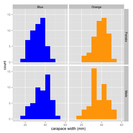
qplot(data = crabs,
      x = Sex, y = FL,
      geom = "boxplot",
      facets = . ~ Species,
      fill = Species, alpha = I(0.8),
      xlab = "",
      ylab = "frontal lobe width (mm)"
      ) +
  theme(legend.position = "none") +
  scale_fill_manual(values = c("blue", "orange"))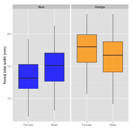
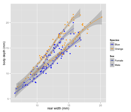
qplot(data = crabs,
      x = RW, y = BD,
      geom = c("point", "smooth"),
      color = Species,
      shape = Sex,
      linetype = Sex,
      xlab = "rear width (mm)",
      ylab = "body depth (mm)"
      ) +
  scale_color_manual(values = c("blue", "orange"))